Freezing panes will make your life a whole lot easier.
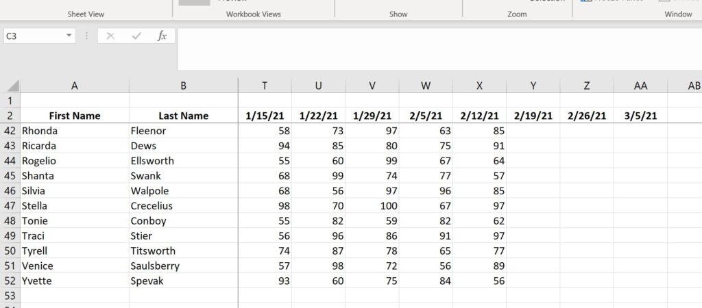
Anytime you have a spreadsheet that is too big to fit on one screen, you have a problem. When you scroll down, you can’t see the column headers. And when you scroll to the right, you can’t see the row labels.
You end up having to scroll back and forth so you know where you’re entering data.
This is confusing, frustrating, a big waste of time, and often leads to errors as you enter data in the wrong cell.
But there’s an easy solution to this: Freezing panes.
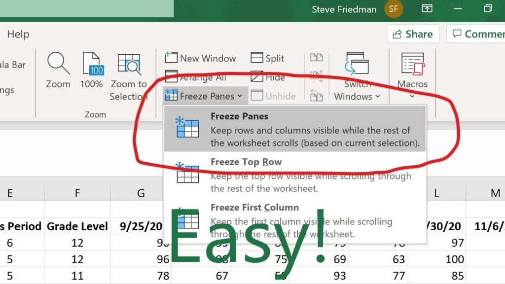
Simply click in the cell below and to the right of your label rows and columns.
Then go to the View ribbon, select the Freeze Panes drop-down, then Freeze Panes.
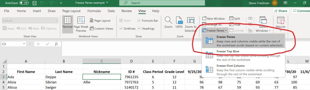
This will keep your label rows and columns visible as you scroll.
And that’s it!
Be sure to check out our blog post/video on Filters: Excel’s Easy Button.